PR2AR_Primer
PR2AR_Primer.RmdMotivation
Plasmodium falciparum parasite rate (\(Pf\)PR) – the proportion of the population testing positive for malaria – is the most frequently measured and estimated malaria metric, making it familiar to both modelers and policy makers. Despite its ubiquity, \(Pf\)PR has substantial limitations as intelligence for policy development. Primarily, a given level of \(Pf\)PR can be associated with a variety of transmission intensities based on differing levels of immunity, multiplicity of infection, case detection rates, vector control, age of infections, among other factors. The attack-rate, \(A(t)\), measures the probability of acquiring an infection during a time period of length \(t\). By developing an algorithm to simulate the latent attack-rate associated with a given time-series of \(Pf\)PR, we enable investigation of risk of malaria infection. Measuring attack-rate – or force of infection (FoI) – directly requires cohort studies which are not universally available and can be expensive to conduct. Deriving estimates of attack-rate from \(Pf\)PR with uniform methods allows for comparison of risk of malaria infection across locations and over time.
A Bad Start
We assume that infections arise from a Poisson process with a rate equal to the FoI, \(h\), so that the probability of acquiring a new infection after \(t\) days is \(A(t) = 1 - e^{-ht}\). Let \(Q(r, t) = e^{-r t}\) denote the fraction of a cohort with recovery rate, \(r\), that naturally remains infected after \(t\) days. It is tempting to start with the simple model: \[\begin{equation} X_{t+1} = A_t (1 - X_t) + Q X_t \end{equation}\] From this, we can solve for \(A_t\): \[\begin{equation} A_t = \frac{X_{t+1} - Q X_t}{1-X_t} \end{equation}\] At the steady state, \(X_{t+1} = X_t,\) so we get the relationship: \[\frac{A}{1-Q} = \frac{X}{1-X}\] Note that \(A\), a probability, can be at most 1, so \(X \leq 1/(2-Q)\). If we take a 14-day time step and assume \(r = \frac{1}{200}\), then we get that Equation 2 gives nonsensical results for \(X > 0.93\). Since there is no evidence that being infected protects against future infection, this is an artifact.
A Better Start
We don’t want to work around artifacts, so what if we rethink the model. What if anyone can get infected, including the fraction that would have otherwise cleared their infections? The susceptible class is \(1-X_t + (1-Q)X_t\), or more simply: \[\begin{equation} X_{t+1} = A_t (1 - Q X_t) + Q X_t \end{equation}\] When \(A=1\), at the steady state, we get that \(X=1\).
Matrix Form
One more wrinkle might help us write down equations without making errors. We will write down equations that assign a state to every person.
\[\begin{equation} \begin{array}{rl}
S_{t+1} &= (1-A_t) S_t + (1 - A_t)(1-Q)X_t\\
X_{t+1} &= A_t S_t + A_t(1 - Q)X_t + Q X_t \\
\end{array} \end{equation}\]
Which we can rewrite in Markov matrix form, ensuring that all entries are positive and every column adds to 1. Let \(Y = \left<S,X\right>\), then we can rewrite these equations as \(Y_{t+1} = B Y_t\) where \[\begin{equation} B= \left[ \begin{array}{cc} 1-A_t & (1-A_t)(1-Q) \\ A_t & A_t(1 - Q) + Q \\ \end{array} \right] \end{equation}\] and we simply check to make sure all the columns sum to 1 to verify that \(B\) is row stochastic. We really wish to solve for \(A_t\), so we write \(Y_{t+1} = A_t W Y_t + V Y_t\), where
\[\begin{equation} W= \left[ \begin{array}{cc} -1 & -(1-Q)\\ 1 & 1 - Q \\ \end{array} \right] \end{equation}\] and \[\begin{equation} V = \left[ \begin{array}{cc} 1 & 1-Q \\ 0 & Q \\ \end{array} \right] \end{equation}\]
Steady State
\(B\) is a Markov matrix, which guarantees that the largest eigenvalue must equal 1 and the associated first right eigenvector, \(x_R\), is the stable equilibrium for the state vector \(Y\), such that \(B x_R = x_R\). We use this to solve for the steady state attack-rate associated with a given \(Pf\)PR value.
Solving for the first right eigenvector \[ (B - I) \cdot Y = \left[ \begin{array}{cc} -A & (1-A)(1-Q) \\ A & -(1-A)(1-Q)\\ \end{array} \right] \cdot Y = A S - (1 - A)(1 - Q)X = 0 \] and including the fact that the sum of all states is 1 \[S = 1 - X\] we get that \[ X^* = \frac{A}{1-Q(1-A)} \] and \[ A^* = \frac{X - QX}{1-QX}\]
Alternatively, we can utilize a one dimensional optimization function to solve: \[A^* = argmin_{A \in [0,1]} f(A) = |X - D Y_{eq}(A)|\] where \[Y_{eq}(A) = (A W + V) x_R = x_R\]
## Solve for steady states using eigen function and algebraic solution
# Set up example B
dt = 10 # ten day time step
r = 1 / 200 # two hundred day duration of malaria infection
Q = exp(-r*dt)
A = 0.1
PAR = list(A = A, Q = Q)
makeB <- function(PAR) {
    A = PAR$A
    Q = PAR$Q
    cbind(c(1 - A, A), c((1 - A)*(1 - Q), A*(1 - Q) + Q))

}
findYeq <- function(PAR, Bfn) {
    B = Bfn(PAR)
    e = eigen(B)
    first = Re(e$vectors[ ,1])
    Yeq = as.vector(first / sum(first))
    return(Yeq)
}
Yeq1 = findYeq(PAR, makeB)
Yeq1
#> [1] 0.3050417 0.6949583

# Find steady state algebraically
algebYeq <- function(PAR) {
    A = PAR$A
    Q = PAR$Q
    X = A / (1 - Q*(1 - A))
    S  = 1 - X
    Yeq = c(S,X)
    return(Yeq)
}
Yeq2 = algebYeq(PAR)
Yeq2
#> [1] 0.3050417 0.6949583

# Confirm steady state
B = makeB(PAR)
sum(B %*% Yeq1 - Yeq1)
#> [1] 0
sum(B %*% Yeq2 - Yeq2)
#> [1] 5.551115e-17

# Convert attack-rate to equilibrium PR
AR2PR <- function(A, PAR, Bfn, eigen = T) {
    PR = c()
    for(Ai in A) {
        PAR$A = Ai
        if(eigen) {
            PRi = findYeq(PAR, Bfn)[2]
        } else {
            PRi = algebYeq(PAR)[2]
        }
        PR = c(PR, PRi)
    }
    return(PR)
}

# Plot
A = seq(0, 1, 0.05)
X = AR2PR(A, PAR, makeB)
plot(A, X, type = "l")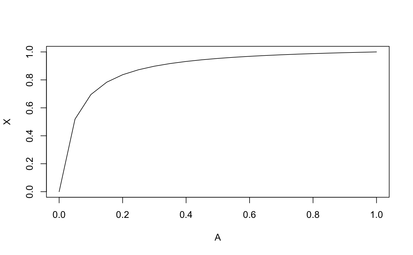
## Solve for attack-rate from X using optimize function and algebraic solution
# optimize function
X = c(0.5, 0.6)
fn <- function(A, PAR, Bfn, X) {
    PR = AR2PR(A, PAR, Bfn)
    return(abs(X - PR))
}
optimA <- function(X, PAR, Bfn) {
    A <- c()
    for(Xi in X) {
        Ai <- optimize(fn, c(0, 1), PAR = PAR, X = Xi, Bfn = Bfn)$minimum
        A <- c(A, Ai)
    }
    return(A)
}
optimA(X, PAR, makeB)
#> [1] 0.04648978 0.06817784

# Algebraic solution
algebA <- function(X, PAR) {
    Q = PAR$Q
    A = (X - Q*X)/(1 - Q*X)
    return(A)
}
algebA(X, PAR)
#> [1] 0.04650262 0.06816891
## Make plots
X = seq(0, 1, 0.05)
A1 <- optimA(X, PAR, makeB)
A2 <- algebA(X, PAR)
plot(X, A1, ylab = "A")
lines(X, A2)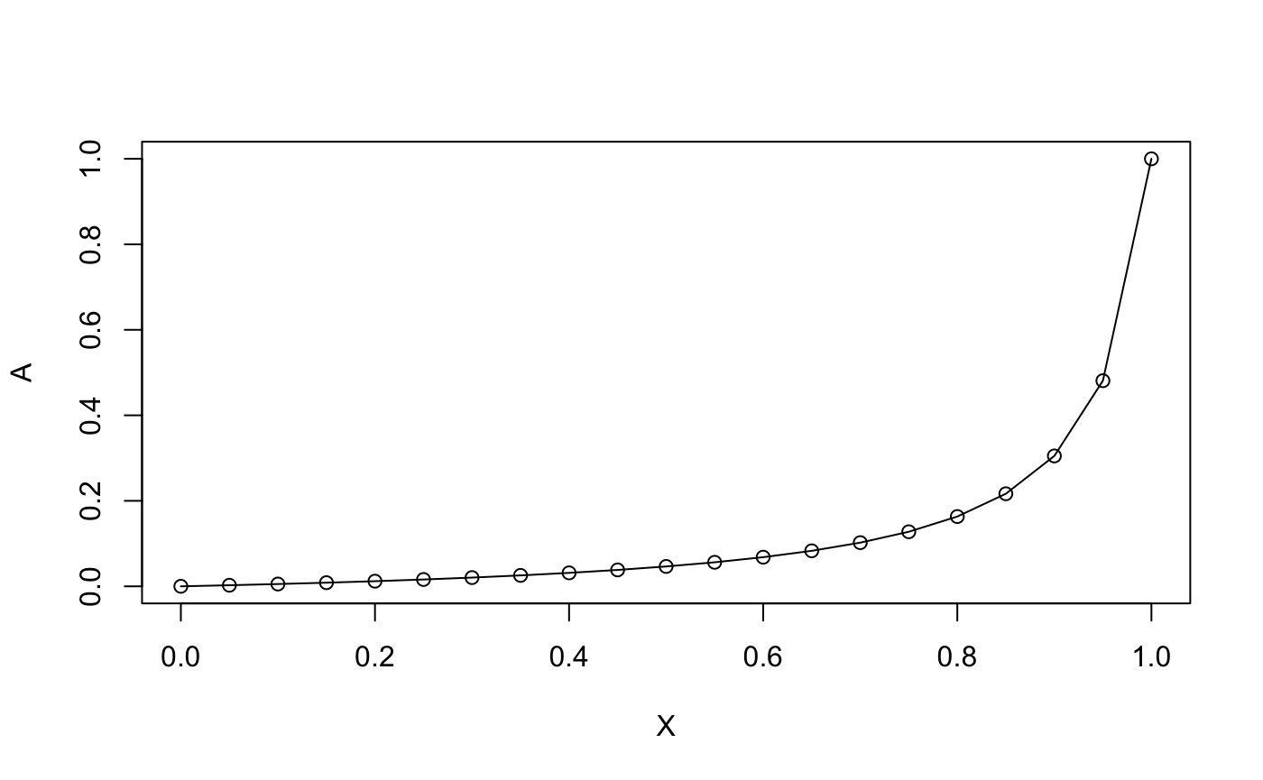
Forward Simulation vs. Steady State
Of course, we don’t know \(Y_t\) but we do know \(X_t\), estimated \(Pf\)PR at time \(t\). We let \(D\) denote the row vector that maps \(Y\) onto \(X\): \(D = \left<0,1 \right>\) and \[X = D \cdot Y = \left[ \begin{array}{cc} 0 & 1 \end{array} \right] \cdot \left[ \begin{array}{c} S\\ X\\ \end{array} \right] \] To solve for the scalar \(A_t\), we simply solve the two-step equation \[D Y_{t+1} = D B Y_t = D \left( A_t W Y_t + V Y_t \right),\] so \[A_t = \left( X_{t + 1} - D V Y_t \right) / \left( D W Y_t \right).\]
This enables an inductive procedure where we only need to estimate an initial state vector, \(Y_0\), and attack-rate, \(A_0\), and all future values can be calculated sequentially… like dominoes!
## Compare steady state solutions to forward simulation
D = t(c(0, 1))
X = c(seq(0.3, 0.6, 0.01), seq(0.59, 0.3, -0.01))
# Find steady state values for X
steadyA = optimA(X, PAR, makeB)

# Generate W and V matrices
makeW <- function(PAR) {
    Q = PAR$Q
    cbind(c(-1, 1), c(-(1 - Q), (1 - Q)))
}
W = makeW(PAR)
makeV <- function(PAR) {
    Q = PAR$Q
    cbind(c(1, 0), c(1 - Q, Q))
}
V = makeV(PAR)

# Set up equilibrium start values
forwardA = PAR$A =c(steadyA[1])
Y = algebYeq(PAR)
# Simulate forward
for(i in 2:length(X)) {
    forwardA[i] = PAR$A = as.numeric((X[i] - D%*%V%*%Y) / (D%*%W%*%Y))
    B = makeB(PAR)
    Y = B%*%Y
}

# Plot
plot(steadyA, type = "l", ylab = "A",
     ylim = c(min(c(steadyA, forwardA)), max(c(steadyA, forwardA))))
lines(forwardA, lty = "dashed")
legend("topleft", legend = c("Steady", "Forward"), lty = 1:2)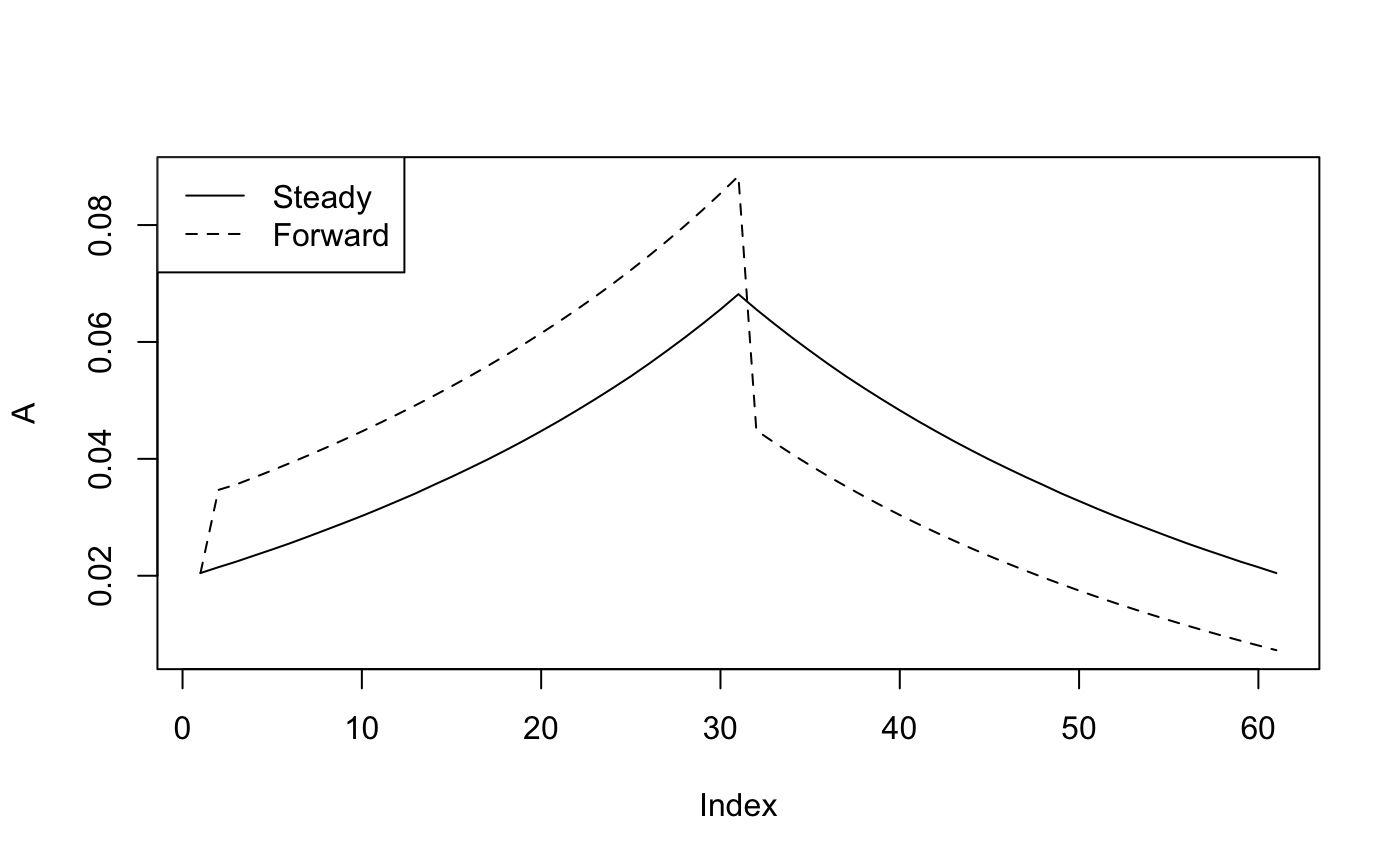
Adding Drugs
Let \(\rho\) denote the fraction of incident malaria infections that are treated and cured. Let \(\delta\) denote the rate anti-malarial drugs are used without a confirmed malaria case attributable to malaria. \(C\) is now a state variable denoting the proportion of the population on treatment.
\[\begin{equation} \begin{array}{rl} S_{t+1} &= (1-\delta)(1-A_t) S_t + (1-A \rho)(1-Q) X_t + (1-\delta) C_t \\ X_{t+1} &= (1-\rho) A_t S_t +(1-\delta)(1-A \rho) Q X_t \\ C_{t+1} &= (\delta + (1-\delta)\rho A_t ) S_t + (\rho A_t + \delta) X_t + \delta \end{array} \end{equation}\]
Now, \(Y = \left<S,X,C \right>\), \(D = \left<0,1,0 \right>\) and \[\begin{equation} B= \left[ \begin{array}{ccc} (1-\delta)(1-A_t) & (1-\delta)(1-A_t \rho)(1-Q) & 1 - \delta \\ (1-\delta)(1-\rho) A_t & (1-\delta)(1-A_t \rho) Q & 0 \\ \delta + (1-\delta)\rho A_t & \delta + (1-\delta)\rho A_t & \delta\\ \end{array} \right] \end{equation}\]
\[\begin{equation} W= (1-\delta)\left[ \begin{array}{ccc} -1& -\rho(1-Q) & 0 \\ 1-\rho & - \rho Q & 0 \\ \rho & \rho & 0 \\ \end{array} \right] \end{equation}\]
\[\begin{equation} V = (1-\delta) \left[ \begin{array}{ccc} 1 & 1-Q & 1 \\ 0 & Q & 0 \\ \delta / (1 - \delta) & \delta / (1 - \delta) & \delta / (1 - \delta)\\ \end{array} \right] \end{equation}\]
Solving for \(Y\) at equilibrium is now critical because there are two unknowns, namely \(S\) and \(C\), for a given value of \(X\).
## Solve for steady states using eigen function and algebraic solution
# Set up example B
PAR$d = 0.05 # rate of anti-malarial drug user w/0 confirmed malaria
PAR$rho = 0.1# fraction of incident malaria cases that are treated and cured
makeBdrugs <- function(PAR) {
    A = PAR$A; Q = PAR$Q; d = PAR$d; rho = PAR$rho
    cbind(c((1 - d)*(1 - A), (1 - d)*(1 - rho)*A, d + (1 - d)*rho*A),
          c((1 - d)*(1 - A*rho)*(1 - Q), (1 - d)*(1 - A*rho)*Q, d + (1 - d)*rho*A),
          c(1 - d, 0, d))
}
colSums(makeBdrugs(PAR))
#> [1] 1 1 1
Yeq = findYeq(PAR, makeBdrugs)
Yeq
#> [1] 0.89224423 0.05710104 0.05065473

# Confirm steady state
B = makeBdrugs(PAR)
sum(B %*% Yeq - Yeq)
#> [1] 5.551115e-17

## Make plots comparing to no treatment
simpleA = PR2AReq(X, PAR, makeB)
drugsA = PR2AReq(X, PAR, makeBdrugs)
plot(steadyA, type = "l", ylab = "A",
     ylim = c(min(c(simpleA, drugsA)), max(c(simpleA, drugsA))))
lines(drugsA, lty = "dashed")
legend("topleft", legend = c("Simple Model (SM)", "SM with Drugs"), lty = 1:2)
# Update AR2PR to accomodate treatment class
AR2PR <- function(A, PAR, Bfn, eigen = T) {
    PR = c()
    for(Ai in A) {
        PAR$A = Ai
        if(eigen) {
            eq = findYeq(PAR, Bfn)
        } else {
            eq = algebYeq(PAR)
        }
        PR = c(PR, eq[2])
        if(length(eq) == 3) {
            if(Ai == A[1]) {
                C = c(eq[3])
            } else {
                C = c(C, eq[3])
            }
        }
    }
    if(length(eq) == 3) {
        out.list = list(X = PR, C = C)
    } else {
        out.list = list(X = PR)
    }
    return(out.list)
}

## Plot for a range of treatment rates
plotAR2PR <- function(PAR, Bfn, AR_range = c(0.01, 1), logX = T, logY = F,
                      plotC = T, plotXover1_C = F) {
  # Prep data
  AR = seq(AR_range[1], AR_range[2], length.out = 100)
  rho = c(seq(0, 0.075, 0.025), seq(0.1, 0.8, .1))
  dt <- data.table()
  for(rho_i in rho) {
    PAR$rho <- rho_i
    PR <- AR2PR(AR, PAR, Bfn)
    X_i = PR$X
    C_i = PR$C
    add.dt <-  data.table(AR = AR, rho = rho_i, X = X_i, C = C_i)
    dt <- rbind(dt, add.dt)
  }

  # Plot
  gg <- ggplot(dt, aes(x = AR, y = X)) + geom_line() + facet_wrap(~rho) +
    theme_classic() +
      labs(title = "Steady-state attack-rate and PfPR for different case management rates",
           subtitle = paste0("Anti-malarial drug use w/o confirmed malaria: ", PAR$d)) +
    xlab("Attack-rate") + ylab("PfPR")
  if(logX) {
    gg = gg + scale_x_continuous(trans='log10')
  }
  if(logY) {
    gg = gg + scale_y_continuous(trans='log10')
  } else {
    gg = gg + ylim(c(0, 1))
  }
  if(plotC) {
    top.dt <- copy(dt)[, C := 0]
    top.dt <- top.dt[nrow(top.dt) - 1:nrow(top.dt) + 1]
    poly.dt <- rbind(dt, top.dt)
    gg = gg + geom_polygon(data = poly.dt, aes(x= AR, y = (1-C), fill = "Treated"), alpha = 0.5) +
         theme(legend.position="bottom", legend.title = element_blank())
  }
  if(plotXover1_C) {
    gg = gg + geom_line(aes(x = AR, y = X / (1 - C)), color = "red")
  }
  gg
}

plotAR2PR(PAR, makeBdrugs)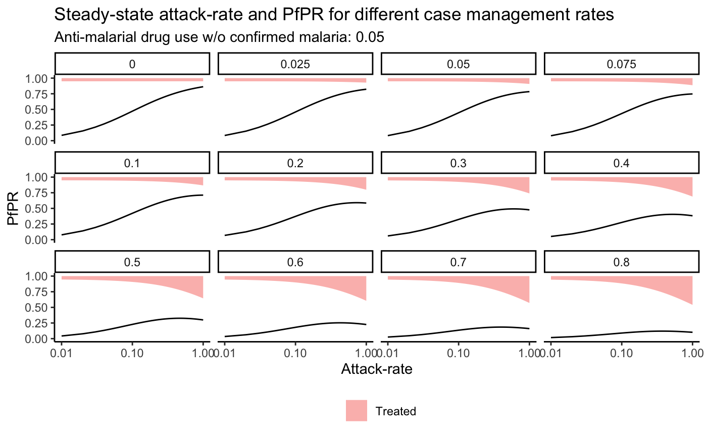
\(Pf\)PR Thresholds and AR2PR Monotonicity
As can be seen in the preceding plots, for a given level of drug use there are levels of \(Pf\)PR that are not plausible. These thresholds can assist with identifying a disconnect between estimated case management and \(Pf\)PR. In addition, the relationship between AR and PR is not monotonic for certain levels of treatment, leading to two solutions for a given \(Pf\)PR that exceeds the PR associated with an AR of 1 but is less than the maximum allowable PR. In order to address both of these problems we will introduce boundary conditions and report both possible AR values when converting from \(Pf\)PR to AR.
AR2PRopt <- function(A, PAR, Bfn) {
  AR2PR(A, PAR, Bfn)$X
}

findAXmax <- function(PAR, Bfn) {
  opt <- optimize(AR2PRopt, interval = c(0, 1), PAR, Bfn, maximum = T)
  A = opt$maximum
  X = opt$objective
  return(list(A = A, X = X))
}

PAR$rho = 0.5
max = findAXmax(PAR, makeBdrugs)
max
#> $A
#> [1] 0.4677827
#>
#> $X
#> [1] 0.3259383

fn <- function(A, PAR, Bfn, X) {
    PR = AR2PR(A, PAR, Bfn)$X
    return(abs(X - PR))
}

PR2AReq <- function(X, PAR, Bfn) {
  A1X <- AR2PR(1, PAR, Bfn)
  max <- findAXmax(PAR, Bfn)
  print(paste0("max A: ", round(max$A, 3), "; max X: ", round(max$X, 3)))
  mono <- abs(A1X$X - max$X) < 0.001
  if(mono) {
    print("Monotonic")
  } else {
    print("Non-monotonic")
    outA2 <- c()
    outY2 <- matrix(nrow = nrow(Bfn(PAR)), ncol = length(X))
  }
  outA <- c()
  outY <- matrix(nrow = nrow(Bfn(PAR)), ncol = length(X))
  for(Xi in X) {
    if(Xi > max$X) {
      outA <- c(outA, NA)
      outA2 <- c(outA2, NA)
      next
    }
    A = optimize(fn, c(0, max$A), PAR = PAR, X = Xi, Bfn = Bfn)$minimum
    outA = c(outA, A)
    PAR$A = A
    Y = findYeq(PAR, Bfn)
    outY[, which(X == Xi)] = Y
    if(!mono) {
      if(Xi > A1X$X) {
        A = optimize(fn, c(max$A, 1), PAR = PAR, X = Xi, Bfn = Bfn)$minimum
        outA2 <- c(outA2, A)
        PAR$A = A
        Y = findYeq(PAR, Bfn)
        outY2[, which(X == Xi)] <- Y
      } else {
        outA2 <- c(outA2, NA)
      }
    }
  }
  if(mono) {
    outList = list(A = outA, Y = outY)
  } else {
    outList = list(A = outA, Y = outY, A2 = outA2, Y2 = outY2)
  }
  return(outList)
}

# Simulate X that exceeds PfPR(A=1) and maximum PfPR
X = seq(0.05, 0.35, 0.01)
X = (1 + 0.1*sin(seq(0, length(X), length.out = length(X))))*X
plot(X, type = "l")
abline(h = max$X, col = "red")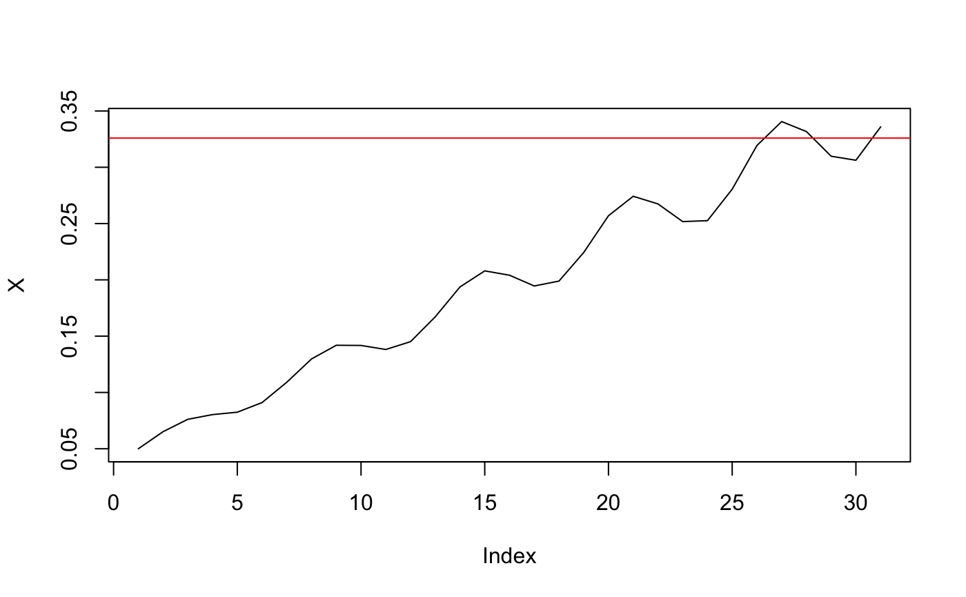
eqAR = PR2AReq(X, PAR, makeBdrugs)
#> [1] "max A: 0.468; max X: 0.326"
#> [1] "Non-monotonic"
eqAR
#> $A
#>  [1] 0.01198213 0.01618449 0.01948225 0.02076928 0.02145081 0.02424543
#>  [7] 0.03058186 0.03871652 0.04404433 0.04393387 0.04236533 0.04548629
#> [13] 0.05659793 0.07270503 0.08300557 0.08007853 0.07329988 0.07630647
#> [19] 0.09666807 0.13284356 0.15987869 0.14836690 0.12603847 0.12705906
#> [25] 0.17195397 0.32290314         NA         NA 0.26098140 0.24517938
#> [31]         NA
#>
#> $Y
#>            [,1]       [,2]       [,3]       [,4]       [,5]       [,6]
#> [1,] 0.89458213 0.87765431 0.86513887 0.86042490 0.85796580 0.84814120
#> [2,] 0.05004153 0.06509816 0.07615038 0.08029452 0.08245216 0.09104262
#> [3,] 0.05537634 0.05724753 0.05871075 0.05928058 0.05958204 0.06081618
#>            [,7]       [,8]       [,9]      [,10]      [,11]      [,12]
#> [1,] 0.82729529 0.80309214 0.78859152 0.78888227 0.79305507 0.78483261
#> [2,] 0.10910224 0.12975252 0.14194077 0.14169783 0.13820470 0.14507580
#> [3,] 0.06360247 0.06715534 0.06946772 0.06941989 0.06874024 0.07009159
#>           [,13]      [,14]      [,15]      [,16]      [,17]      [,18]
#> [1,] 0.75797138 0.72458183 0.70598491 0.71107851 0.72345485 0.71786177
#> [2,] 0.16715745 0.19370522 0.20797962 0.20411018 0.19458147 0.19890933
#> [3,] 0.07487118 0.08171294 0.08603547 0.08481131 0.08196368 0.08322889
#>           [,19]     [,20]     [,21]     [,22]     [,23]     [,24]
#> [1,] 0.68397785 0.6366700 0.6087158 0.6200009 0.6445785 0.6433669
#> [2,] 0.22431573 0.2569425 0.2742311 0.2674562 0.2517593 0.2525611
#> [3,] 0.09170642 0.1063876 0.1170531 0.1125429 0.1036622 0.1040720
#>          [,25]     [,26] [,27] [,28]     [,29]     [,30] [,31]
#> [1,] 0.5977265 0.5043288    NA    NA 0.5354249 0.5446465    NA
#> [2,] 0.2805385 0.3193380    NA    NA 0.3097963 0.3062571    NA
#> [3,] 0.1217350 0.1763332    NA    NA 0.1547788 0.1490964    NA
#>
#> $A2
#>  [1]        NA        NA        NA        NA        NA        NA        NA
#>  [8]        NA        NA        NA        NA        NA        NA        NA
#> [15]        NA        NA        NA        NA        NA        NA        NA
#> [22]        NA        NA        NA        NA 0.6775987        NA        NA
#> [29] 0.8384780 0.8925494        NA
#>
#> $Y2
#>      [,1] [,2] [,3] [,4] [,5] [,6] [,7] [,8] [,9] [,10] [,11] [,12] [,13]
#> [1,]   NA   NA   NA   NA   NA   NA   NA   NA   NA    NA    NA    NA    NA
#> [2,]   NA   NA   NA   NA   NA   NA   NA   NA   NA    NA    NA    NA    NA
#> [3,]   NA   NA   NA   NA   NA   NA   NA   NA   NA    NA    NA    NA    NA
#>      [,14] [,15] [,16] [,17] [,18] [,19] [,20] [,21] [,22] [,23] [,24]
#> [1,]    NA    NA    NA    NA    NA    NA    NA    NA    NA    NA    NA
#> [2,]    NA    NA    NA    NA    NA    NA    NA    NA    NA    NA    NA
#> [3,]    NA    NA    NA    NA    NA    NA    NA    NA    NA    NA    NA
#>      [,25]     [,26] [,27] [,28]     [,29]     [,30] [,31]
#> [1,]    NA 0.3993442    NA    NA 0.3696145 0.3609016    NA
#> [2,]    NA 0.3193404    NA    NA 0.3097930 0.3062515    NA
#> [3,]    NA 0.2813154    NA    NA 0.3205924 0.3328469    NA
In the above PR2AR function we are returing the equilibrium AR associated with each \(Pf\)PR value. While this is a helpful approximation, as we would expect (and demonstrated earlier) the forward simulation estimates of AR differ from the equilibrium estimates.
makeBdrugs <- function(PAR) {
    A = PAR$A; Q = PAR$Q; d = PAR$d; rho = PAR$rho
    cbind(c((1 - d)*(1 - A), (1 - d)*(1 - rho)*A, d + (1 - d)*rho*A),
          c((1 - d)*(1 - A*rho)*(1 - Q), (1 - d)*(1 - A*rho)*Q, d + (1 - d)*rho*A),
          c(1 - d, 0, d))
}
# Generate W and V matrices
makeWdrugs <- function(PAR) {
    A = PAR$A; Q = PAR$Q; d = PAR$d; rho = PAR$rho
    cbind(c(-(1 - d), (1 - d)*(1 - rho), (1 - d)*rho),
          c(-(1 - d)*rho*(1 - Q), -(1 - d)*rho*Q, (1 - d)*rho),
          c(0, 0, 0))
}
W = makeWdrugs(PAR)
makeVdrugs <- function(PAR) {
    PAR$A = 0
    makeBdrugs(PAR)
}
V = makeVdrugs(PAR)

D= t(c(0, 1, 0))

# Set up equilibrium start values
forwardA = PAR$A =c(eqAR$A[1])
Y = findYeq(PAR, makeBdrugs)
# Simulate forward
for(i in 2:length(X)) {
    forwardA[i] = PAR$A = as.numeric((X[i] - D%*%V%*%Y) / (D%*%W%*%Y))
    B = makeBdrugs(PAR)
    Y = B%*%Y
}

# Plot
plot(eqAR$A, type = "l", ylab = "A",
     ylim = c(0, max(c(eqAR$A, forwardA), na.rm = T)))
abline(h = max$A, col = "red")
lines(forwardA, lty = "dashed")
legend("topleft", legend = c("Steady", "Forward"), lty = 1:2)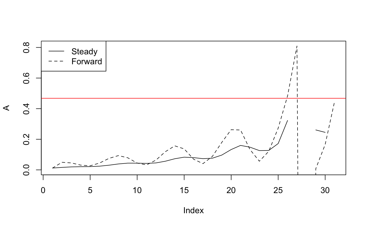
Having worked through all that, we jump to a much harder model tracking the age of infection with the possibility of superinfection.
Age of Infection (AoI) and Overwriting Superinfection
We keep most of the notation from before, but now let \(I_{i,t}\) denote the fraction of the population that has had its most recent infection \(i\) months ago, and \(E_{i,t}\) denote the fraction of the population that was just exposed and whose previous infection occurred \(i\) months ago: \[\begin{equation} \begin{array}{rl} S_{t+1} & = (1-A_t) S_t + \sum_i (1-A_t)(1-Q_i) I_{i,t} \\ E_{0, t+1} &= A_t \left[ S_t + \sum_i (1-Q_i)I_{i,t} \right] \\ E_{1,t+1} &= A_t \left[E_{0,t} + \sum_{i=1}^n E_{i,t}) \right] \\ E_{i,t+1} &= A_t Q_{i-1} I_{i-1,t} \\ E_{n,t+1} &= A_t \left( Q_{n-1, t} I_{n-1,t} + Q_{n, t} I_{n,t} \right) \\ I_{1,t+1} &= (1-A_t) \sum_{i=1}^n E_{i,t}\\ I_{i,t+1} &= (1-A_t) Q_{i-1, t} I_{i-1,t} \\ I_{n,t+1} &= (1-A_t) \left( Q_{n-1, t} I_{n-1,t} + Q_{n, t} I_{n,t} \right) \\ \end{array} \end{equation}\] …so we write \[ Y = \left<S, E_0, E_i, \ldots, E_{n-1}, E_n, I_1, I_i, \ldots, I_{n-1}, I_n \right> \] and \[ D = \left<0, 0, 1, \ldots, 1\right> \]
PAR$In <- 5
PAR$Cn <- 0
makeD <- function(PAR) {
  In = PAR$In; Cn = PAR$Cn
  D = c(0)
  if(In > 0) {
    D = c(D, 0, rep(1, In*2))
  } else {
    D = c(D, 1)
  }
  D = c(D, rep(0, Cn))
  return(D)
}
makeD(PAR)
#>  [1] 0 0 1 1 1 1 1 1 1 1 1 1

makeBage <- function(PAR) {
  A = PAR$A; Q = PAR$Q; In = PAR$In
  S = c(S=1-A, E0=A, E=rep(0, In), I = rep(0,In))
  E0 = c(0, 0, A, rep(0, In-1), (1-A), rep(0, In-1))
  M = cbind(S, E0)

  Ei = E0
  for(i in 1:In) M = cbind(M, Ei)

  for(i in 1:(In-1)){
    Ii= c((1-A)*(1-Q), A*(1-Q), rep(0,i), A*Q, rep(0, In-i-1), rep(0,i), (1-A)*Q, rep(0, In-i-1))
    M = cbind(M, Ii)
  }

  Im= c( (1-A)*(1-Q), A*(1-Q), rep(0,In-1), A*Q,  rep(0,In-1), (1-A)*Q)
  M = cbind(M, Im)

  M
}
B = makeBage(PAR)
colSums(B)
#>  S E0 Ei Ei Ei Ei Ei Ii Ii Ii Ii Im
#>  1  1  1  1  1  1  1  1  1  1  1  1

makeVage <- function(PAR) {
  PAR$A=0
  makeBage(PAR)
}
V = makeVage(PAR)
colSums(V)
#>  S E0 Ei Ei Ei Ei Ei Ii Ii Ii Ii Im
#>  1  1  1  1  1  1  1  1  1  1  1  1

makeWage <- function(PAR){
  (makeBage(PAR)-makeVage(PAR))/PAR$A
}
W = makeWage(PAR)
colSums(W)
#>            S           E0           Ei           Ei           Ei
#> 1.110223e-16 1.110223e-16 1.110223e-16 1.110223e-16 1.110223e-16
#>           Ei           Ei           Ii           Ii           Ii
#> 1.110223e-16 1.110223e-16 6.938894e-18 6.938894e-18 6.938894e-18
#>           Ii           Im
#> 6.938894e-18 6.938894e-18

# Update AR2PR to accomodate exposure and treatment class
AR2PR <- function(A, PAR, Bfn, eigen = T) {
    D = makeD(PAR)
    PR = c()
    for(Ai in A) {
        PAR$A = Ai
        if(eigen) {
            eq = findYeq(PAR, Bfn)
        } else {
            eq = algebYeq(PAR)
        }
        PR = c(PR, D%*%eq)
        if(PAR$Cn > 0) {
            Ci = sum(eq[(length(eq) - 1:PAR$Cn) + 1])
            if(Ai == A[1]) {
                C = c(Ci)
            } else {
                C = c(C, Ci)
            }
        }
    }
    if(length(eq) == 3) {
        out.list = list(X = PR, C = C)
    } else {
        out.list = list(X = PR)
    }
    return(out.list)
}

findAXmax(PAR, makeBage)
#> $A
#> [1] 0.9999323
#>
#> $X
#> [1] 0.9999967

X = seq(0.5, 0.8, 0.01)
X = (1 + 0.1*sin(seq(0, length(X), length.out = length(X))))*X
plot(X, type = "l")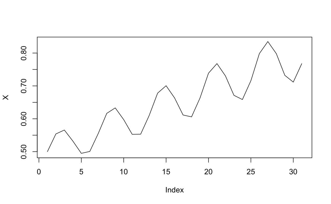
eqAR = PR2AReq(X, PAR, makeBage)
#> [1] "max A: 1; max X: 1"
#> [1] "Monotonic"
plot(eqAR$A, type = "l")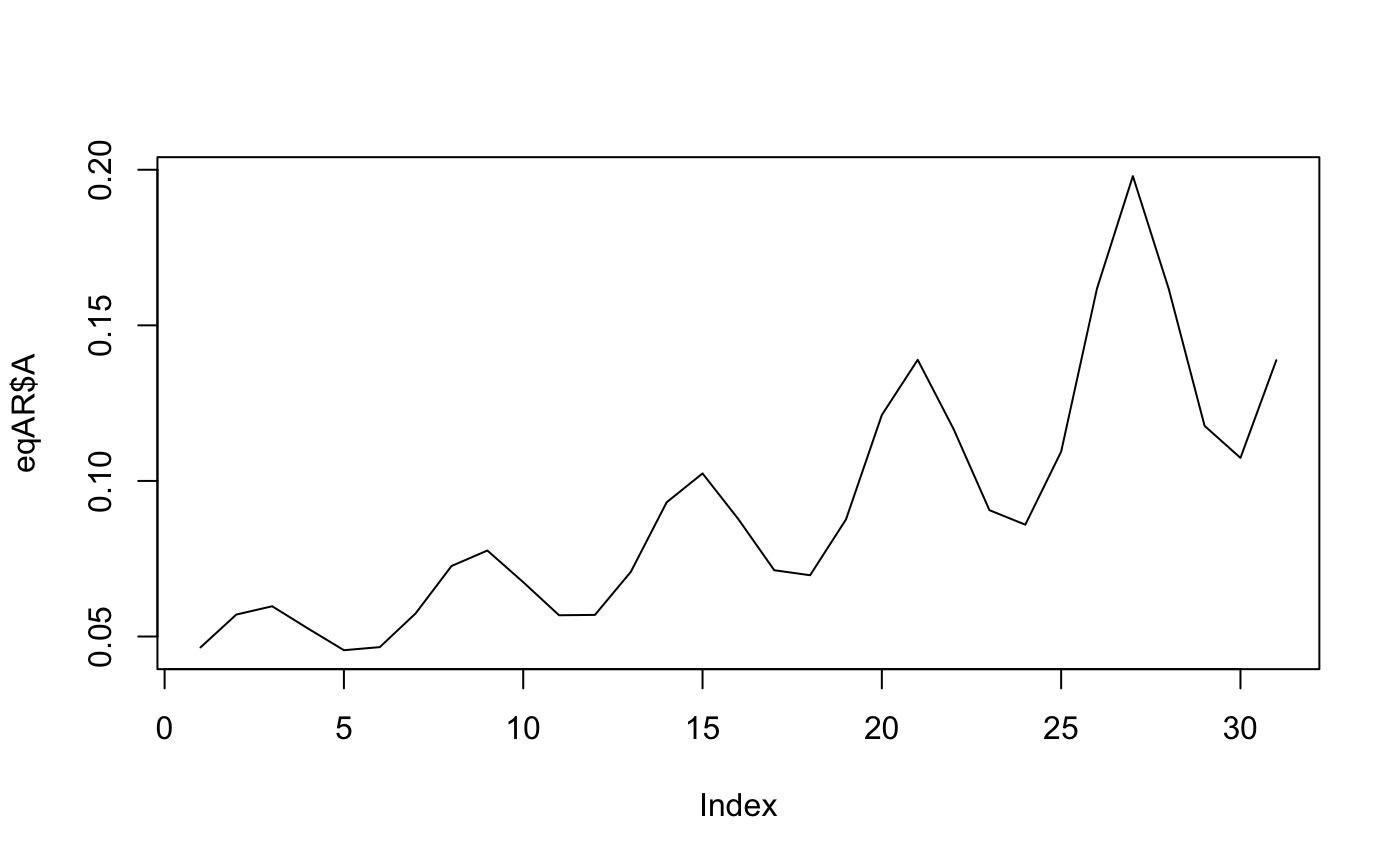
PAR$A =c(eqAR$A[1])
Y = findYeq(PAR, makeBage)
D = makeD(PAR)
as.numeric((X[i] - D%*%V%*%Y) / (D%*%W%*%Y))
#> [1] 5.187568e+16

D%*%W%*%Y
#>              [,1]
#> [1,] 5.161384e-18
AoI Forward Simulation
Forward simulation with the initial \(A_t\) formula breaks down because there is a one timestep delay in the impact of \(A\) on \(X\), so that \(D \cdot W \cdot Y_t = 0\). We reformulate \(A_t\) as a function of \(X_{t+2}\);
\[D Y_{t+2} = X_{t+2} = D B_{t+1} B_{t} Y_t = D(A_{t+1}W + V)(A_t W + V) Y_t = D(A_t A_{t+1} W^2 + A_{t+1} W V + A_t V W + V^2) Y_t\]
Because the row sums of \(W\) are zero, the terms \(A_t A_{t+1} W^2\) and \(A_{t+1} W V\) drop out and we get,
\[ A_t = \frac{X_{t+2} - D V^2 Y_t} {D V W Y_t}\]
## Update
fn2 <- function(params, PAR, Bfn, X) {
  A1 = params[1]
  A2 = params[2]
  D = makeD(PAR)
  PAR$A = A1
  Y0 = findYeq(PAR, Bfn)
  PAR$A = A2
  B2 = Bfn(PAR)
  Y1 = B2%*%Y0
  Y2 = B2%*%Y1
  return(as.numeric(sum(abs(X[1] - D%*%Y1)) + sum(abs(X[2] - D%*%Y2))))
}

params = optim(fn = fn2, par = c(0, 0.1), PAR = PAR, Bfn = makeBage, X = X)$par

# Set up equilibrium start values
forwardA = PAR$A =c(params[1])
Y0 = findYeq(PAR, makeBage)
forwardA[2] = PAR$A =c(params[2])
B = makeBage(PAR)
Y = B%*%Y0

# Check against input X
D = makeD(PAR)
X[1]
#> [1] 0.5
D%*%Y
#>      [,1]
#> [1,]  0.5
forwardX = c(D%*%Y)

# Simulate forward
for(i in 3:length(X)) {
    forwardA[i] = PAR$A = as.numeric((X[i] - D%*%V%*%V%*%Y) / (D%*%V%*%W%*%Y))
    B = makeBage(PAR)
    Y = B%*%Y
    forwardX = c(forwardX, D%*%Y)
}
sum(abs(X[1:length(forwardX)] - forwardX))
#> [1] 1.147394e-08

# Plot
plot(eqAR$A, type = "l", ylab = "A",
     ylim = c(min(c(eqAR$A, forwardA)), max(c(eqAR$A, forwardA), na.rm = T)))
abline(h = max$X, col = "red")
lines(forwardA, lty = "dashed")
legend("topleft", legend = c("Steady", "Forward"), lty = 1:2)
Combine AoI with Overwriting Superinfection and Drugs
\[\begin{equation} \begin{array}{rl} S_{t+1} & = \left( 1 -\delta \right) \left[ (1-A_t) S_t + \sum_i (1-A_t)(1-P_i) I_{i,t} + C_{2,t}\right] \\ E_{0, t+1} &= \left( 1 -\delta \right) A_t \left[ S_t + \sum_i (1-P_i)(1-\rho_i)I_{i,t} \right] \\ E_{1,t+1} &= \left( 1 -\delta \right) A_t \left[E_{0,t} + \sum_{i=1}^n (1-\rho_i) E_{i,t}) \right] \\ E_{i,t+1} &= \left( 1 -\delta \right) A_t P_{i-1} I_{i-1,t} \\ E_{n,t+1} &= \left( 1 -\delta \right) A_t P_{i-1} (I_{n-1,t} + I_{n,t}) \\ I_{1,t+1} &= \left( 1 -\delta \right) (1-A_t) \sum_{i=1}^n (1-\rho_i) E_{i,t}\\ I_{i,t+1} &= \left( 1 -\delta \right) (1-A_t) P_{i-1, t} I_{i-1,t} \\ I_{n,t+1} &= \left( 1 -\delta \right) (1-A_t) \left( P_{n-1, t} I_{n-1,t} + P_{n, t} I_{n,t} \right) \\ C_{1,t+1} & = (1-\delta) \sum_i \left( \rho_i E_{i, t} + A_t \rho_i I_{i, t}\right) + \delta \\ C_{2,t+1} & = (1-\delta) C_{1,t} \\ \end{array} \end{equation}\] …so we write \[ Y = \left[S, E_0, E_i, \ldots, E_{n-1}, E_n, I_1, I_i, \ldots, I_{n-1}, I_n, C_1, C_2 \right] \] And we can write the previous equations as: \[ Y_{t+1} = (1-\delta) \left[ A_t W Y_t + V Y_t \right]\] where \(W=\) \[(1-\delta) \left[ \begin{array}{c||c|cc|cccc|cc} &S&E_0&E_i&I_1&I_i&I_m&I_n&C1&C2\\ \hline \hline S&-1&0&0&-(1-P_1)&-(1-P_2)&-(1-P_m)&-(1-P_n)&0&0\\ E_0&1&0&0&(1-P_1)(1-\rho_1)&(1-P_i)(1-\rho_i)&(1-P_m)(1-\rho_m)&(1-P_n)(1-\rho_n)&0&0\\ E_1&0&1&(1-\rho_i)&0&0&0&0&0&0\\ E_2&0&0&0&P_1(1-\rho_1)&0&0&0&0&0\\ E_3&0&0&0&0&P_2 (1-\rho_2)&0&0&0&0\\ E_n&0&0&0&0&0&P_m (1-\rho_m)&P_n (1-\rho_n)&0&0\\ I_1&0&-1&-(1-\rho_i)&0&0&0&0&0&0\\ I_2&0&0&0&-P_1&0&0&0&0&0\\ I_3&0&0&0&0&-P_2&0&0&0&0\\ I_n&0&0&0&0&0&-P_m&-P_n&0&0\\ C1&0&0&0&\rho_1&\rho_2&\rho_m&\rho_n&0&0\\ C2&0&0&0&0&0&0&0&0&0\\ \end{array} \right]\]
\(V=\) \[(1-\delta) \left[ \begin{array}{c||c|cccc|cccc|cc} &S&E_0&E_1&E_2&E_n&I_1&I_2&I_m&I_n&C_1&C_2 \\ \hline \hline S&1&0&0&0&0&1-P_1&1-P_2&1-P_m&1-P_n&0&1\\ \hline E_0&0&0&0&0&0&0&0&0&0&0&0 \\ E_1&0&0&0&0&0&0&0&0&0&0&0 \\ E_2&0&0&0&0&0&0&0&0&0&0&0 \\ E_3&0&0&0&0&0&0&0&0&0&0&0 \\ E_n&0&0&0&0&0&0&0&0&0&0&0 \\ \hline I_1&0&1&1-\rho_1&1-\rho_2&1-\rho_n&0&0&0&0&0&0 \\ I_2&0&0&0&0&0&P_1&0&0&0&0&0 \\ I_3&0&0&0&0&0&0&P_2&0&0&0&0 \\ I_n&0&0&0&0&0&0&0&P_m&P_n&0&0 \\ \hline C_1&0&0&\rho_1&\rho_2&\rho_n&0&0&0&0&0&0\ \\ C_2&0&0&0&0&0&0&0&0&0&1&0\\ \end{array} \right] + \left[ \begin{array}{c} 0\\0\\0\\0\\0\\0\\0\\0\\0\\0\\0\\\delta/(1-\delta)\\0 \end{array} \right]\]
makeBdrugs_age = function(PAR){
  A = PAR$A; Q = PAR$Q; rho = PAR$rho; In = PAR$In; Cn = PAR$Cn
  S = c(S=1-A, E0=A, E=rep(0, In), I = rep(0,In), C=rep(0,Cn))
  E0 = c(0, 0, (1-rho)*A, rep(0, In-1), (1-rho)*(1-A), rep(0, In-1), rho, rep(0, Cn-1))
  M = cbind(S, E0)

  Ei = E0
  for(i in 1:In) M = cbind(M, Ei)

  for(i in 1:(In-1)){
    Ii= c((1-A)*(1-Q), A*(1-Q), rep(0,i), A*Q, rep(0, In-i-1), rep(0,i), (1-A)*Q, rep(0, In-i-1), rep(0, Cn))
    M = cbind(M, Ii)
  }

  Im= c( (1-A)*(1-Q), A*(1-Q), rep(0,In-1), A*Q,  rep(0,In-1), (1-A)*Q, rep(0, Cn))
  M = cbind(M, Im)

  if(Cn==2){
    C1 = c(0, rep(0, 2*In+1),0,1)
    M = cbind(M, C1)
    C2 = c(1, rep(0, 2*In+1),0,0)
    M = cbind(M, C2)
  }
  M
}

makeV = function(PAR, Bfn){
 PAR$A=0
 Bfn(PAR)
}

makeW = function(PAR, Bfn){
  V = makeV(PAR, Bfn)
 (Bfn(PAR)-V)/PAR$A
}

PAR$Cn = 2
X = seq(0.05, 0.35, 0.01)
X = (1 + 0.1*sin(seq(0, length(X), length.out = length(X))))*X
ARdrugs_age = PR2AReq(X, PAR, makeBdrugs_age)
#> [1] "max A: 0.185; max X: 0.322"
#> [1] "Non-monotonic"
## Generic forward simulation function
simAR <- function(X, PAR, Bfn) {
V = makeV(PAR, Bfn)
W = makeW(PAR, Bfn)
D = makeD(PAR)
outY <- matrix(nrow = length(D), ncol = length(X))
if(PAR$In > 1) {
params = optim(fn = fn2, par = c(0, 0.1), PAR = PAR, Bfn = Bfn, X = X)$par
# Set up equilibrium start values
outA = PAR$A =c(params[1])
Y0 = findYeq(PAR, Bfn)
outA[2] = PAR$A =c(params[2])
B = Bfn(PAR)
Y = B%*%Y0
outY[, 1] = Y
# Simulate forward
for(i in 3:length(X)) {
outA[i] = PAR$A = as.numeric((X[i] - D%*%V%*%V%*%Y) / (D%*%V%*%W%*%Y))
B = Bfn(PAR)
Y = B%*%Y
outY[, i - 1] = Y
}
} else {
# Set up equilibrium start values
forwardA = PAR$A =c(eqAR$A[1])
Y = findYeq(PAR, Bfn)
outY[, 1] = Y
# Simulate forward
for(i in 2:length(X)) {
forwardA[i] = PAR$A = as.numeric((X[i] - D%*%V%*%Y) / (D%*%W%*%Y))
B = Bfn(PAR)
Y = B%*%Y
outY[, i] = Y
}
}
return(list(A = outA, Y = outY))
}
## Set up PR2AR that can take any model and return equilibrium or forward simulation values
PR2AR <- function(X, PAR, eq = F) {
if(PAR$In > 1 & PAR$Cn > 0) {
Bfn = makeBdrugs_age
} else if (PAR$In > 1) {
Bfn = makeBage
} else if (PAR$Cn > 0) {
Bfn = makeBdrugs
} else {
Bfn = makeB
}
if(eq) {
outList <- PR2AReq(X, PAR, Bfn)
} else {
outList <- simAR(X, PAR, Bfn)
}
return(outList)
}
forwardA = PR2AR(X, PAR, eq = F)$A
eqA = PR2AR(X, PAR, eq = T)$A
#> [1] "max A: 0.185; max X: 0.322"
#> [1] "Non-monotonic"
plot(eqA, type = "l", ylab = "A",
ylim = c(min(c(eqA, forwardA), na.rm = T), max(c(eqA, forwardA), na.rm = T)))
abline(h = max$X, col = "red")
lines(forwardA, lty = "dashed")
legend("topleft", legend = c("Steady", "Forward"), lty = 1:2)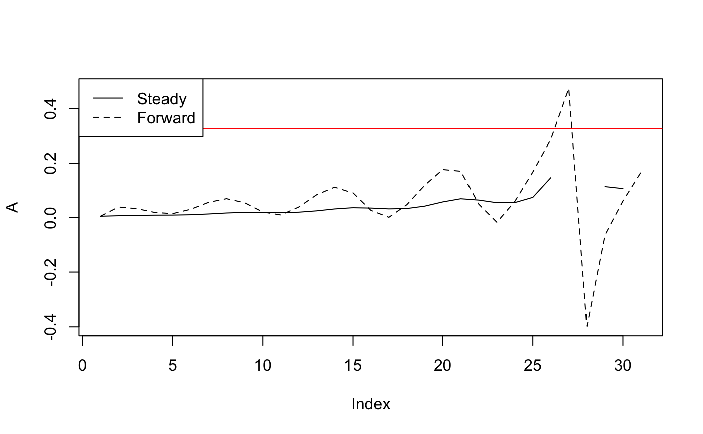
Dynamic Treatment Rates and Generic Solution to Exposure Lags
Rather than forcing treatment rates to be static throughout the simulation, we would rather be able to supply a vector of treatment rates with equal length to input PfPR. This extra layer of complication means that matrices \(V\) and \(W\) are no longer time invariant and must be recalculated at each time step. Furthermore, forward simulation in the presence of an exposure-based lag requires the multiple
\[D Y_{t+2} = X_{t+2} = D B_{t+1} B_{t} Y_t = D(A_{t+1}W_{t+1} + V_{t+1})(A_t W_t + V_t) Y_t = D(A_t A_{t+1} W_{t+1}W_t + A_{t+1} W_{t+1} V_t + A_t V_{t+1} W_t + V_{t+1}V_t) Y_t\]
\[ A_t | \ell = \frac{X_{t+1 + \ell} - D \prod_{i = 0}^{\ell}(V_{t + i}) Y_t} {D \prod_{i = 0}^{\ell - 1}(V_{t + i}) W_t Y_t}\] where \(\ell\) is the length of the lag in time steps.